The purpose of this module is to verify a line or cable model. In many cases when creating a higher frequency model for transient analysis some parameters could be uncertain (especially average ground resistivity and conductor height). Very often the only reliable benchmark data available are the power frequency sequential series impedances and shunt admittances (which even could be based on measurements).
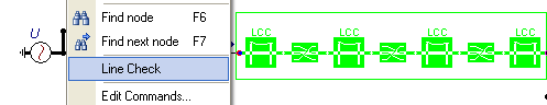
Fig. 1. Selecting a line to verify/check
The user invokes this module by selecting a line/cable in the circuit window and then click on ATP|Line Check. First a dialog box appears where the user can select the input and output nodes. ATPDraw suggests the leftmost nodes as input and the rightmost as output. The number of inputs and outputs must be equal and it is possible to change, add, and delete the default suggestions. In case of 3-phase nodes the user must specify the full single phase names including the ABC or DEF extensions (select ATP|Make Name to identify the node names). The user must also select the frequency where the calculations are performed.
The phase sequence must be the same for the input (left=sending) and output (right=receiving) side. With transposition objects involved, the user might need to correct the phase sequence of the output side to match the input.
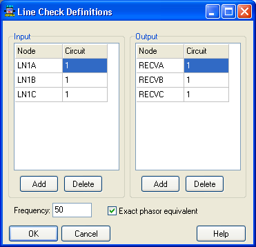
Fig. 2. Selecting the inputs and outputs.
Frequency: Test frequency in Hz.
Assumption: Distributed parameters: Zsc=3Us/(Is+2Ir), Yoc=3Is/(Us+2Ur) as described in the User Manual chapt. 7.2.
PI-equivalent (use this when capacitances are concentrated): Zsc=Us/Ir, Yoc=2Is/(Us+Ur).
Sending end only (same as in LCC|Verify): Zsc=Us/Is, Yoc=Is/Us
Us, Is: Sending end quantities. Ur, Ir receiving end quantities. Zsc remote short-circuited. Yoc remote end open.
Exact phasor equivalent: Insert this card into ATP, uncertain what it actually does.
ATPDraw then creates a file LineCheck.dat in the LCC-directory. For a 3-phase case 4 sequential data cases are created (6-phase: 12 and 9-phase:24 due to mutual coupling effects) positive and zero sequence series impedance (output end grounded) and shunt admittance (output end open). ATPDraw then runs ATP and interprets the LineCheck.lis file. To obtain an approximation for the series impedance and shunt admittance currents and voltages at both ends are monitored and equivalent distributions obtained. See Assumption above.
The results are presented in the Result window. Note the admittance is presented as divided by ω. The results are presented both per phase and (more useful) as symmetrical components. Classical JMarti models might give inaccurate results for power system steady-state testing. The embedded JMarti model based on vector fitting improved this in most cases.
It is possible to create a text file of the results.
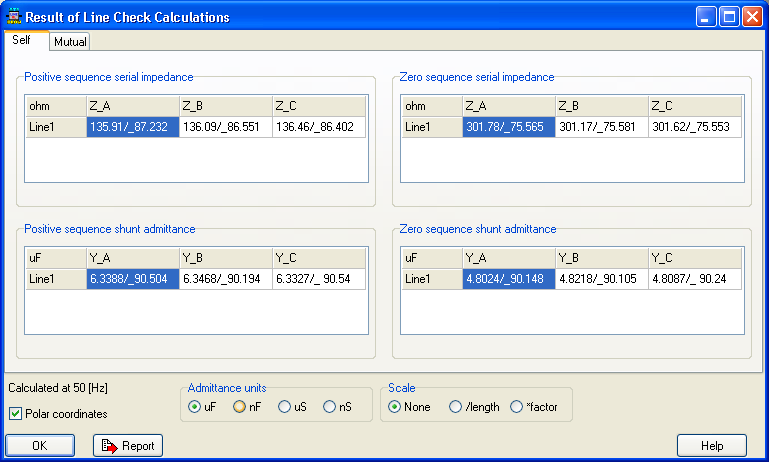
Fig. 3. Results of the line check calculations.