By checking the "Internal calculation" button the line and cable modeling, ATPDraw's internal Line Constants and Cable Parameters routines are used. This is a completely new feature in ATPDraw v7.4 and a perfect handling of all aspects is likely missing. The internal calculations are without any third-party dependencies and are fast (typically a few seconds). Understand that line and cable modeling are highly complex processes that involve intricate Bessel function formulations, eigenvalue analysis of complex, asymmetrical and frequency dependent matrices, lease square fitting problems etc. [1, 2, 3]. In some cases ATPDraw could manage to find a model where ATP fails (for instance in larger Enclosing Pipe cases) and probably vice versa. Part of the reason and difficulty is degenerated eigenvalues (with unresolved switchover) and collapsing eigenvectors in certain frequency ranges [1]. Lots of effort has been invested in treatment of (nearly) perfect symmetrical cases but this tends to be harder the larger the system becomes. The main intention of the new module is for research where high accuracy is needed. Comparison with the native ATP routines is always recommended.
The main advantage of the internal routines are:
•They are thread-safe and no disk interaction is used in the process. There is potential for a significant speed-up in multiple runs and utilization of multiple cores also for transmission line simulations. This applies in particular to PI-equivalents (and Bergeron).
•Vector fitting [3] is used for JMarti models and this significantly improves their low frequency response. Verify and Line Check now shows far better agreement with PI-equivalent for the same frequency.
•Universal Line Model [4] is introduced that for the first time enables highly accurate cable models directly embedded in ATPDraw. This is particularly important for mutual effects in cable systems.
•Import of Z- and Y-matrices from external sources and internal modeling (PI, Bergeron, JMarti and ULM). An XML-format is defined that allows import of Z and Y as function of frequencies from for instance FEM solvers. Vector Fitting is used to fit the elements of Z and Y to rational functions to enable re-sampling of the data.
•For Cable Parameters, conductors can be both in air and ground. The initial choice of cables in air/ground is just used to define the sign of vertical position. If cables in air is chosen, a negative sign of vertical position means the cable is in ground.
•The MoM-SO method for proximity effect correction in pipe type cables is supported.
•The internal routines will open doors to further development into ground return modeling, mutual coupling between overhead and underground conductors and handling of proximity effect.
The following limitations exist in ATPDraw v7.4:
•Cable Constants is not supported, only Cable Parameters. The main difference is the logic for conductor grounding, but also the cascaded PI option.
•Verify Line Model Frequency Scan will compare the new models with ATP's LCC parameters. Far more useful visualizations of the fitting of the characteristic admittance Yc and the propagation matrix H (and their modes) are shown instead under Verify for JMarti and ULM lines.
•The ULM uses a TYPE94 MODELS approach and work only for a single model (several equal sections can be used) and without AC-initialization.
•Line Constant is developed with skin effect calculation and the REACT option does not work as intended yet.
•Output of matrices and diagnosis is limited.
•Testing special or extreme cases. Bessel functions are tricky is practice and users should stay within the range 1 Hz - 1 MHz. Extreme values of conductivity, frequency and permeability could in theory be problematic even if series/asymptotic expansions are used. The common practice for JMarti lines to specify a very low initial frequency is not beneficial anymore and not recommended. In close to symmetrical cases "Unresolved eigenvalue switchover" error messages could show up and this in general makes good fitting impossible. Difficult situations are transposed/symmetrical systems with slightly different internal impedance, and the user should thus check if different parameters are given to conductors by a mistake. Cables with floating sheaths inside a pipe are also problematic (this applies to ATP as well).
Some minor differences in the impedances are observed compared to ATP's supporting routines. The main reason is the modeling of the ground return impedance for overhead lines. While ATP uses Carson's approximations [5], ATPDraw uses the complex skin depth formulation for overhead lines and approximations (according to Saad, Gaba, Giroux) recommended in [6] for cables. Exact integral methods recommended in [1] will be investigated in the future. The coupling between cables inside a finite pipe follows the refined summation formulas analyzed in [7]. For Auto-bundling, multiple conductors are introduced and eliminated, the concept of geometric mean radius is not used.
JMarti lines/cables:
•The modes of the characteristic impedance Zc and the modes of the propagation matrix H are fitted with Vector Fitting [3]. Travel times are identified by the imaginary part of the eigenvalues at high frequency in addition to the minimum phase shift approach [8].
•Initial real poles are distributed logarithmically spaced up to 1e4/tau and not relocated by Vector Fitting. Poles are allowed to be complex conjugated but forced into real poles by the method proposed in [9]. Then residues are calculated (JMarti models require reals poles and residues only). Fitting the modes very accurately is of limited value since a constant (and real) transformation matrix is used in the end anyway.
•The user can control the maximum number of poles and the fitting accuracy, but default settings could mostly be left unchanged.
•Stay within the 1 Hz - 1 MHz range. The number of frequency points per decade is recommended to be around 10.
•The Matrix frequency should be selected around the dominant frequency response of the study.
•After the fitting, ATPDraw reports the average fitting of Yc and H and values in pu and below 0.01 is typically achieved.
•Mutual coupling in cable systems will still not be accurate as small elements in the H-matrix will be poorly represented by a constant transformation matrix.
•Significant improvements can be expected in studies where the combination of power frequency and high frequency is of important (which is most cases) and significant improvements are achieved when comparing JMarti lines and PI-equivalents calculated at the test frequency.
Universal Line Models (ULM) [4]:
•The trace of the characteristic admittance matrix Yc and the modes of H are fitted with Vector Fitting [3] with real and complex conjugated poles [4]. Travel times are identified by the imaginary part of the eigenvalues at high frequency in addition to the minimum phase shift approach [8] without optimization.
•The model is applied directly in the phase domain via state-space implementation in TYPE94 MODELS code [10]. No transformation matrix is used as the ULM model is in the phase domain.
•ULM is supported in two ways. As introduced in Version 7.4 as an internal MODELS Type 94 component (single instance restriction and slow performance) and as a Foreign Model according to [12] (multiple instance support and fast performance). The Foreign Model approach requires a special, compiled ATP-solver that must be enabled under the ATP Connection Wizard (F10).
•Stay within the 1 Hz - 1 MHz range. The number of frequency points per decade is recommended to be around 10.
•The Velocity frequency should be large (typically 1 MHz). The original ULM paper [4] used this for approximating of the modes of H with a constant eigenvector matrix to reduce the eigenvalue switchover problem. This must not be confused with the JMarti approach.
•The user can control the maximum number of poles and the fitting accuracy, but default settings could mostly be left unchanged. Significantly fewer poles are needed compared to the JMarti model.
oThe fitting routine will always start with Ymin and Hmin number of poles and move towards Ymax, Hmax to obtained the requested accuracy epsY and epsH (given in %). For repeated attempts where the numbers of poles are know, the user can force this by setting Ymin=Ymax=Yknown and Hmin=Hmax=Hknown. This will speed up the fitting process.
oOne of the settings EpsDeg (default 10 degrees) controls the merging of modes: If the product of travel time difference and maximum frequency Δτ*fmax < EpsDeg*pi/180 the modes will be merged. If poor fit is obtained (at low-frequency typically), EpsDeg could be reduced to increase the number of active modes.
•Mutual coupling in cable systems will now be highly accurate.
•Steady-state initialization is not supported at this stage. Frequency scan (performed by ATP) will probably never be supported.
•Instability could occur if fitting at low frequency is not sufficiently accurate. The interpolation method reported in [11] is implemented in the Foreign Model.
•The ULM model requires a large number of residues for the fitting of H and this can result in memory allocation problems in MODELS, but not in the Foreign Model implementation. The model shown in Fig. 1 and 2 required 360 residues for the Yc matrix and 1944 residues for the H matrix.
•Figure 1 shows the fitting plot that appears in Verify for the cable system reported in [4]. The time domain step response of the induced voltage on the neighbor screen and core at the far end is shown in Figure 2.
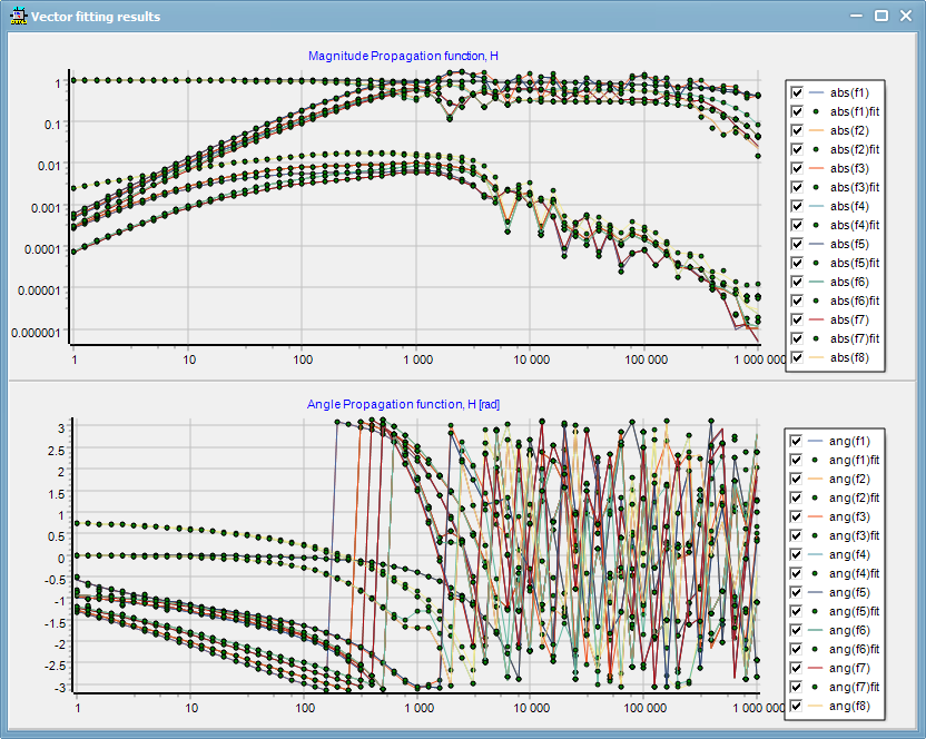
Figure 1. Fitting of 6 conductor, 10 km cable system in ATPDraw using Vector Fitting. Geometry according to [4]. Solid lines is the propagation matrix H and the dots represent the fitting (10 points per decade). All 36 elements of H are shown in the figure.
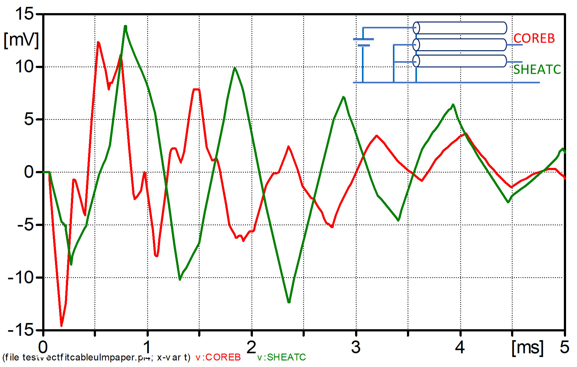
Figure 2. Step response of 10 km long single core cables. Geometry according to [4].
Matrix Import:
Supported only with "Internal calculation" checked.
The user must select NumPhases action before import with three possibilities:
•The imported file determines the number of phases.
•The model as specified above determines the number of phases and the matrices in the file are either reduced (normal case, conductors above NumPhases given by model are assumed to be on ground potential carrying current) or
•ignored (the conductors above NumPhases are assumed to be on ground potential carrying zero current (same as segmented ground in Line Constants)).
The following (case sensitive) XML-format is defined:
<ZY NumPhases="3" Length="1" ZFmt="R+Xi" YFmt="C">
<Z Freq="10">
0.001+0.001i, 0.001+0.001i, 0.001+0.001i
0.001+0.001i, 0.001+0.001i, 0.001+0.001i
0.001+0.001i, 0.001+0.001i, 0.001+0.001i
</Z>
<Z Freq="1000">
0.1+0.1i, 0.1+0.1i, 0.1+0.1i
0.1+0.1i, 0.1+0.1i, 0.1+0.1i
0.1+0.1i, 0.1+0.1i, 0.1+0.1i
</Z>
//Etc. in increasing order of frequency. Typically 3 points per decade are needed in the frequency range of interest.
<Y Freq="1">
0.1e-6, -0.01e-6, -0.01e-6
-0.01e-6, 0.1e-6, -0.1+0.1
-0.01e-6, -0.01e-6, 0.1e-6
</Y>
</ZY>
ZFMt can be ["R+Xi", "R+iX", "R+Xj", "R+jX"], YFmt can be ["C", "G+Bi", "G+iB", "G+Bj", "G+jB"].
With YFmt=C" the (Maxwell) capacitance is given in Farad, frequency does not matter in this case.
The frequency points must be the same for Z and Y (unless YFMt="C" is used).
Length="1" means data per meter length.
The curves for Z and Y are shown on the Data page.
The models PI, Bergeron, JMarti and ULM can be selected. JMarti and ULM will require Z and Y given at selected points in the frequency range of interest. This would also be needed for PI and Bergeron unless the exact desired frequency point is provided. Vector Fitting is used to approximate the elements in Z and Y with rational functions sum(c/(s-a))+d for resampling.
References:
[1] T. Noda: "Numerical Techniques for Accurate Evaluation of Overhead Line and Underground Cable Constants", IEEJ Trans, 2008.
[2] A. Ametani: "A general formulation of impedances and admittance in cables", IEEE Power App. Syst., 1980.
[3] B. Gustavsen, A. Semlyen: "Rational approximation of frequency domain responses by vector fitting", TRPWD 1999.
[4] A. Morched, B. Gustavsen, M. Tartibi: "A universal model for accurate calculation of electromagnetic transients on overhead lines and underground cables", TRPWD, 1999.
[5] H. Dommel: "EMTP Theory book", 1987.
[6] Juan A. Martinez Velasco (ed) :"Power system transients: Parameter determination", Ed. 1, CRC Press, 2010.
[7] H. K. Høidalen: "Analysis of Pipe-type Cable Impedance Formulations at Low Frequencies", TRPWD, 2013.
[8] B. Gustavsen: "Optimal time delay extraction for transmission line modeling", TRPWD 2017.
[9] E.S. Bañuelos-Cebral et.al. "Accuracy enhancement of the JMarti model by using real poles through vector fitting", Electrical Engineering, 2019.
[10] H. K. Høidalen, A. H. Soloot: ""Cable modelling in ATP - from NODA to TYPE94", EEUG meeting 2010, Helsinki.
[11] B. Gustavsen: "Avoiding numerical instabilities in the universal line model by two-segment interpolation scheme", TRPWD 2013.
[12] F. O.S. Zanon, O. E.S. Leal, A. De Conti: "Implementation of the universal line model in the alternative transients program", EPSR, 2021.