Besides the standard components, the user can create his/her own control modules using the MODELS simulation language in ATP [4]. ATPDraw supports only a simplified usage of MODELS. The user writes a model-file and ATPDraw takes care of the INPUT/OUTPUT section of MODELS along with the USE of each model. The following restriction applies:
•Only INPUT, OUTPUT and DATA supported in the USE statement. Not possible with expressions, call of other models or specification of HISTORY or DELAY CELLS under USE
Using this feature requires knowledge about the syntax and general structure of MODELS language. There are two options for creating a model object in ATPDraw:
•Create a script internally (or load a .mod file created externally) and rely on ATPDraw for automatic identification and layout/icon. The icon and node positions can later be fine tuned. This is the preferred option.
•Create a template manually under Library | Template on disc | New Model sup-file and a corresponding .mod file.
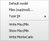
Options under the MODELS sub-menu.
Default model
This will load a simple, default object and display it in the circuit window. Its input dialog box will look as shown in Fig. 4.76 (2 data, 4 nodes). Click on the Edit button to show the Models Editor and modify the script directly or to import a script from file or clipboard. Click on Done in the main menu of the Models Editor when finished. ATPDraw will then identify the object and create the required template, including icon, see Fig. 4.77. Inputs and outputs are placed to the left and right of the icon, respectively. You can whenever you want go back and modify the script, and if you change the number of input and outputs the icon will be recreated. The Models Editor support syntax highlighting, code folding, context menu (right click) insert of most language feature, and a simple debugging. ATPDraw will correctly identify array INPUT, OUTPUT and DATA when the first index is unity MYDATA[1..24], MYINPUT[1..3] (for INPUT/OUTPUT there is a upper limit of 26, A..Z phase extension) etc.
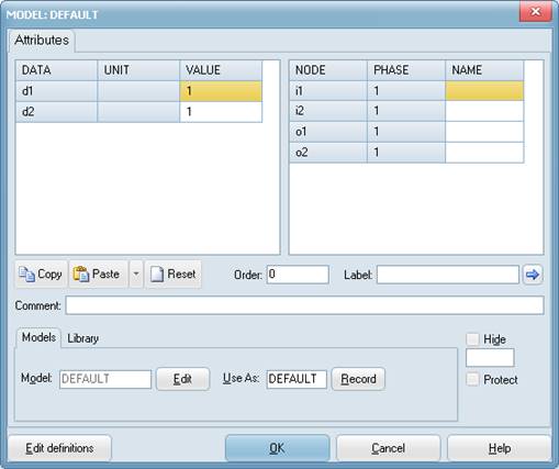
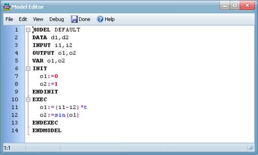
Model component dialog box. And Text Editor
Files (sup/mod)...
Selecting MODELS | Files (sup/mod)... in the component selection menu performs an Open Model dialog box where the user can choose a model file name or a support file name. These files are normally stored under the \MOD folder. If a .mod file was selected ATPDraw interprets the file as shown in Fig. 4.77 and a model component with the corresponding definition and icon appears. If a support file with the same name as the model file exist in the same folder, this file is used instead as basis for the model definitions. In this case the new model object appears immediately in the circuit window, i.e. the Information dialog shown in Fig. 4.77 does not show up.
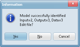
Interpretation of the model.
The Component dialog of model objects has a new input section Models below the DATA and NODES attributes as shown in Fig. 4.78. This new section has two fields: Model which is disabled (but automatically follows what is defined in the Model text found using the Edit button) and a Use As field for specification of the model_name in the USE model AS model_name statement of MODELS. The Record button is used for output of internal model variables. On the Library page the link to the original support file on disk is given and a Reload option is made available. Remember that the original support file on disk not necessarily match the present Model text if the user has changed this.
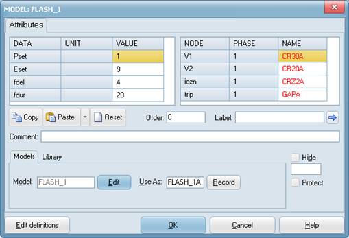
The component dialog box of model object FLASH_1 .
The input/output to MODELS, the use of the model and interfacing it with the rest of the circuit are handled by ATPDraw, automatically. Model descriptions are written directly in the ATP file instead of using $Include. Blank lines are removed when inserting the model file in the ATP-file. The general structure of the MODELS section in the .atp input file is shown below:
MODELS
/MODELS
INPUT
IX0001 {v(CR30A)}
IX0002 {v(CR20A)}
IX0003 {v(CRZ2A)}
OUTPUT
GAPA
MODEL FLASH_1
------------------------------------------
Description of the model is pasted here
------------------------------------------
ENDMODEL
USE FLASH_1 AS FLASH_1
INPUT
V1:= IX0001
V2:= IX0002
iczn:= IX0003
DATA
Pset:= 1.
Eset:= 9.
Fdel:= 4.
Fdur:= 20.
OUTPUT
GAPA:=trip
ENDUSE
ENDMODELS
Type 94
Selecting MODELS | Type 94|THEV, ITER, NORT, NORT-TR will load a corresponding default model component. You can then open the component which will bring up the Type 94 component dialog box as shown in Fig. 4.79. As for simple models you can then click on the Edit button to inspect or modify the type 94 models text. When you click on Done in the Text Editor ATPDraw tries to identify the model and then displays a message box similar to Fig. 4.77. Be aware of that the name of the models must be six characters or less. The bottom section of the input dialog has to the right four radio buttons: THEV, ITER, NORT and NORT-TR for specification of the solution method for ATP when interfacing the Type-94 object with the rest of the electrical network. The Data, Node fields and the icon will update dependent on the choice of type. You can also specify the number of phases (#Ph: 1..26) in the component. Branch output and Record of internal variable are also available.
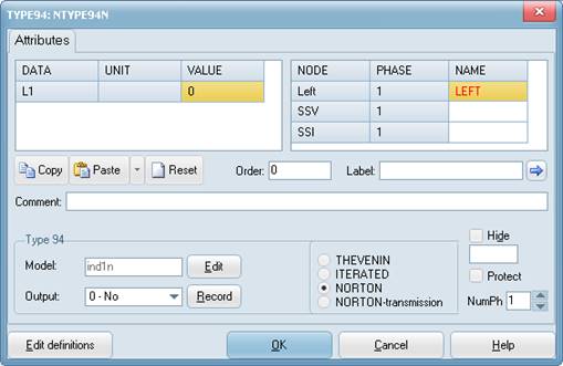
Component dialog box of Type-94 model objects.
Signal input and data values for a Type-94 object are loaded by ATP and the output of the object are also used automatically by ATP. Interfacing it with other components of the circuit is handled by ATPDraw. A Type-94 compatible .mod files must have a fixed structure and the use of such an object also requires special declarations in the ATP input file as shown next:
Structure of a Type-94 compatible script:
MODEL ind1n
comment ----------------------------------------------------------------
| Internal circuit: 1-ground : L1 | | |
| 1 o | |
| - ground |
| Built for use as a 1-phase non-transmission type-94 Norton component |
------------------------------------------------------------- endcomment
comment ----------------------------------------------------------------------
| First, declarations required for any type-94 iterated model |
| (the values of these data and input are loaded automatically by ATP) |
| (the values of these outputs are used automatically by ATP) |
| (DO NOT MODIFY THE SEQUENCING OF THE DATA, INPUT, AND VAR IN THIS GROUP) |
| (the names may be modified, except 'n') ‘ ’ |
| (when built for n=1, the array notation is not required) |
------------------------------------------------------------------- endcomment
DATA n -- number of phases
ng {dflt: n*(n+1)/2} -- number – conductances
INPUT v -- voltage(t) at terminal 1
v0 -- voltage(t=0) at terminal 1
i0 -- current(t=0) into terminal 1
VAR i -- current(t) into terminal 1
is -- Norton source(t+timestep) at terminal 1
g -- conductance(t+timestep) at terminal 1
flag -- set to 1 whenever a conductance value is modified
OUTPUT i, is, g, flag
comment ----------------------------------------------------------------------
| Next, declarations of user-defined data for this particular model |
| (values which must be defined when using this model as a type-94 component) |
------------------------------------------------------------------- endcomment
DATA L1 -- [H] reference value of inductance L
comment ----------------------------------------------------------------------
| Next, declarations private to the operation of this model |
------------------------------------------------------------------- endcomment
VAR st -- used for converting Laplace s to time domain
L -- [H] variable value of inductance L
INIT
st := 2/timestep -- trapezoidal rule conversion from Laplace
L := L1 -- initialize variable inductance value
g:= 1/(st*L) -- conductance converted from Laplace 1/sL
ENDINIT
EXEC -- L is constant in this example
IF t=0 THEN
flag := 1 -- conductance values have been changed
i := i0 -- t=0 current through L
is := -i0 -g*v0 -- –istory term for next step
ELSE
flag := 0 -- reset flag
i := g*v -is -- –pplying trapezoidal rule, calculate from v(t)
is := -i -g*v --–history term from trapezoidal rule, for next step
ENDIF
ENDEXEC
ENDMODEL
The use of a Type-94 Norton model in the ATPDraw generated input file is shown next.
C Time varying inductor
94LEFT IND1N NORT 1
>DATA L1 0.1
>END
Write Max/Min
This is a special cost function or reporting component using Models. The component extracts a value from a simulation by reading from the LIS file. As default the minimum or maximum value of a single input signal is extracted, but the user can add more sophistication to this. Only the signal after a user selectable time Tlimit is identified. The component supports multiple run via the Sidebar or ATP|Settings/Variables and contains a View module for displaying the result. A data parameter AsFuncOf can be used to pass a loop variable from the Variables (if a number is specified here, the simulation number is used instead). The component is used extensively in circuit optimization and can extract results of systematic parameter variations, see Chapt. 5.9.
Extract1/Extract1 (new in version 7.4)
Record the extremal value of simulations within a Tstart, Tstop span and scale, store and optionally write the value(s) for one selected simulation on screen. The component has the same capabilities as WriteMaxMin when it comes to tracking multiple-run extremal values, but is more powerful as it has a Tstop criterion, scaling and 3-phase and on-screen capabilities.
Write MonteCarlo
Uses the same approach as WRITEMAXMIN and extracts data from the LIS-file. Accumulates extremal values from Monte Carlo studies in statistical probability density function with user specified resolution.