The core model is connected to the artificial winding on the core surface. This 3-phase node is labeled C and it also available externally for measurement of the voltage and flux linkage.
The implementation of the core model is performed by the master student Nicola Chiesa during the spring of 2005. Only stacked cores with three and five legs are supported at this point as shown in fig. 1. Basically the inductive and resistive core parts are treated independently. The core losses are at this point assumed to be linear and the nonlinear inductances are modelled by the Frolich equation. Each part of the core is modelled with its own core loss resistance and nonlinear inductance using information about their relative cross section and length to scale the values.
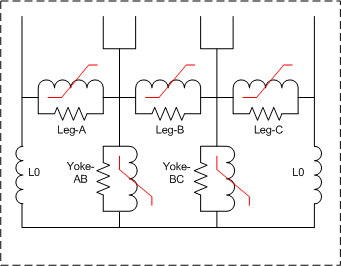
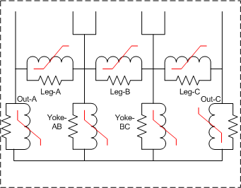
Fig. 1a) 3-legged stacked core. Fig. 1b) 5-legged stacked core.
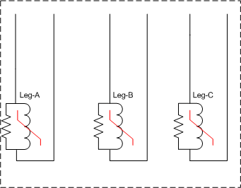
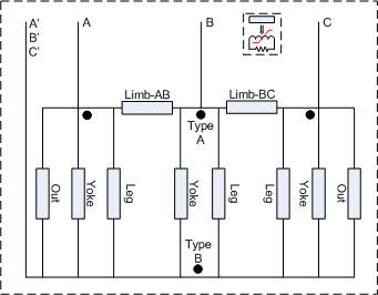
Fig. 1c) Triplex core. Fig. 1d) Shell-form core.
It is assumed that the magnetic material is characterized by four parameters a, b, d and e. A library of typical steel materials is developed (ARMCO M2, M4 and M6, NIPPON M4 and M6, and METGLASS 2605TCA). This list is based on fitting the manufacturer's data from state of the art catalogs. Older steel materials will have a different characteristic and the losses are typically higher. The material library will be used for design data and typical values.
The B/H relation ship is assumed to follow the Frolich equation ![]() and the specific loss is assumed to follow
and the specific loss is assumed to follow![]() , f is the power frequency.
, f is the power frequency.
The specific loss is traditionally (for instance Westinghouse T&D reference book, 1964) assumed to be ![]() with x said to be 3 for modern materials in the year of 1964. In the above expression t is the thickness of the laminates. The traditional expression was tested on modern material data with little success.
with x said to be 3 for modern materials in the year of 1964. In the above expression t is the thickness of the laminates. The traditional expression was tested on modern material data with little success.
Fig. 2 shows the fit of the specific losses and DC-magnetization curve of ARMCO M4 steel. The Frolich fitting is not very good, and in fig. 6b) fitting around the knee point (nominal flux) was preferred at the sacrifice of high field fitting (B=1.9 T). Similar fitting is performed for the other core materials.
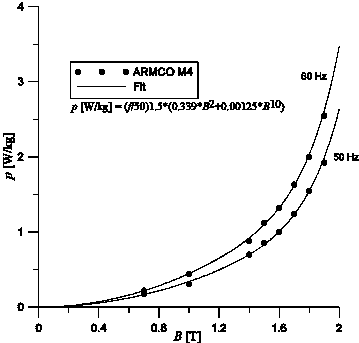
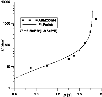
Fig.2 a) Core loss curves Fig. 2 b) DC-magnetization curve
The essence of the inductive core modelling is to obtain the three values a', b' and (optionally) c' in the Frolich equation for the l/i-characteristic by an optimization technique. The modified Frolich equation is implemented in ATPDraw as a part of Nicola Chiesa's work is on the form:
 .
.
The measured or assumed rms value of the magnetizing current (resistive component subtracted) is compared with a calculated quantity and iterated until a best fit is found. An quasi-Newton (L-BSGF) optimization method is implemented in ATPDraw to minimize the cost function OF:
![]()
Inductance modeling
The basic Frolich equation for the magnetic fields is
 .
.
This equation is scaled to fluxlinkage and current by using l=B*A*N and i=H*N/l. This gives the general flux-linkage current relationship based on the relative core dimensions (Ar and lr) to the leg:

with in the case of design data available

Based on the electrical core model shown in Fig. 1 the the external currents can be found as function of time, and finally the rms value. A part of this process is to determine the voltage/flux at the neutral point of the core. The resisive currents are ignored in this process.
Core loss modeling
The core loss is assumed proportional to the core volume and to the square of the rms voltage across the section (~Steinmetz coefficient n=2).
Triplex: Ploss= 3*Pleg
3-legged: Ploss= (3*Pleg+2*Pyoke) = p*(3+2*Vry*(Uy/U)^2)
5-legged: Ploss= (3*Pleg+2*Pyoke+2*Pout) = p*(3+2*Vry*(Uy/U)^2+2*Vro*(Uo/U)^2))
Shell-form: Ploss= (3*Pleg+3*Pyoke+2*Pout+2*Plimb)
where Vry and Vro are the relative volumes of the yoke and outer legs referred to the main leg
and Uy and Uo are the rms values of the voltages across the yoke and outer leg sections in Fig. 1.
It is assumed that the neutral voltage, Uo, is mainly determined by the dominant inductive currents and this voltage is found by taking the time derivative of the neutral flux found in the Frolich optimization. The yoke voltage, Uy is the rms value of (U-Uo). Since the resistive currents contribute to the current balance in Fig. 1 there will be some unaccuracies in the estimation of core losses of a 3- and 5-legged transformer even at rated voltage.
The total core modeling process is illustrated in fig. 3. From ATPDraw v5.6 a gradient based optimization method is used. This was possible when the final slope inductance was added since this will guarentee a flux value for any current.

Fig. 3. a) Flow chart of magnetizing inductance calculations.
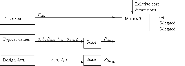
Fig. 3. b) Flow chart of core loss calculations.
Typical values
The estimation of the magnetizing current (Im) is based on table 9, p.83 in MTU7 (from A. Greenwood: Electrical Transients in Power Systems, Wiley 1991). Some fitting of the data is performed which results in
![]() [%] when the basic insulation level (BIL) is known and
[%] when the basic insulation level (BIL) is known and
![]() [%] when BIL must be estimated.
[%] when BIL must be estimated.
BIL is in [kV], u is the rated voltage in [kV] and s is the rated power in [MVA].
For a typical core model the user has to specify the maximum B-field (normally 1.5-1.7 Tesla) and the maximum core loss density. First a core material has to be guessed and this gives the a and b values in the Frolich equation (and possibly also the c and d values that would replace pmax).
The following relations are then assumed:
![]()
![]() which a bit doubtfully assumes a sinusoidal magnetizing current.
which a bit doubtfully assumes a sinusoidal magnetizing current.
This gives the parameter of the flux linkage current characteristic:
![]() and
and ![]()
The core loss is estimated to
![]() where p [W/kg] and r [kg/m3] are given the volume A\\l is estimated.
where p [W/kg] and r [kg/m3] are given the volume A\\l is estimated.
Typical core losses are ignored at the moment.
Test report
The user specifies the excitation voltage in [%], the current in [%] and the core loss in [kW].
The core loss is used directly as explained above to obtain the core resistances. At the moment the core resistances are assumed to be linear and the core loss value at 100 % excitation is used (interpolation implemented if this point is not available).
The inductive magnetizing current for each point is calculated as
 [%]
[%]
This results in a sequence of excitation points (Urms and Irms). If a single point is specified the core is assumed to be linear. If more than one point is specified these are sent to the optimization routine that returns the a' and b' values used to describe the l/i relationship for the core inductances as shown above and in MTU7 eq. (44).
Design data
For design data the user specifies the core material directly with is B/H relationship (a and b values in the Frolich equation). The absolute core dimensions and the number of inner-winding turns N are known, so the inductances can be found directly as
 for the leg
 for the outer leg
 for the yoke
Based on manufacturer data the core losses can be established as
![]()
With ![]() and known values of the core weight (volume and density) the core loss can be calculated.
and known values of the core weight (volume and density) the core loss can be calculated.