1. Lightning induced voltage calculation
In this example a model for induced voltage calculations in overhead lines is presented. The example is taken from [1, 2]. The basic assumptions are:
The overhead line can be treated as loss-less.
The electrical field is assumed to propagate unaffected by the ground.
The Agrawal coupling model is used.
The transmission line (TL) model is used for the lightning channel, assuming a pure step current at ground. The actual current shape at ground is taken into account by a final convolution integral of the induced voltages. This assumption is believed to be valid the first few microseconds where often the maximum induced voltage occurs.
The electrical field from the lightning leader is constant, and the resulting induced voltage is zero.
The same inducing voltage is assumed in all phases, but this could easily be extended since the inducing voltage is proportional to the line height, z.
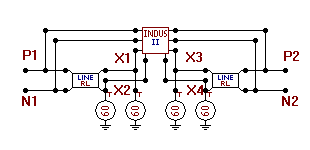
The circuit shown in Fig. 1 shows the equivalent circuit of and overhead line excited inducing fields from a lightning channel. It can be connected to any component in the ATP, and several line segments are allowed.

Fig. 1. Equivalent circuit of 2-phase overhead line, excited by nearby lightning. Modeled in ATPDraw.
Below, an example of the electric circuit part of the two-phase model in Fig. 1 is listed in ATP file format.
/BRANCH
51X1 P1 300.
52X2 N1 200. 500.
51P2 X3 300.
52N2 X4 200. 500.
/SOURCE
60X1
60X2
60X3
60X4
A further simplification of this model is to rewrite it into a type94 Norton-transmission component.
References
[1] H.K. Høidalen, Lightning induced voltages in low-voltage systems, PhD thesis, ISBN 82-471-0177-1, University of Trondheim 1997.
[2] H.K. Høidalen, "Calculation of Lightning-induced Overvoltages using MODELS ", Proc. int. conf on Power Syst. Transients IPST'99, June 20-24, Budapest.
MODEL indloss2 --Calculation of lightning induced voltage in multi-phase overhead line with lossy ground effect
CONST Tmax {VAL:500} --number of time steps
n {VAL:2} --number of phases
c {VAL:3.e8} --speed of light
I0 {VAL:1} --step current ampl.
eps0 {val:8.85e-12} --permittivity
sigma {VAL:0.001} --ground conductivity
epsr {VAL:10} --relative permittivity
tc {VAL:2e-6} --current time to crest
th {VAL:5e-5} --current time to half value
v {VAL:1.5e8} --current velocity
INPUT UA[1..n],UB[1..n] --terminal voltages
DATA XA0,YA0,XB0,YB0 --line position parameters (in meters in a global co-ordinate system)
z[1..n] {DFLT:10} --phase heights
Im {DFLT:3e4} --current amplitude
X0 {DFLT:0.0} --lightning x-pos (in meters in a global co-ordinate system)
Y0 {DFLT:0.0} --lightning y-pos
OUTPUT UrA[1..n],UrB[1..n] --type 60 sources
VAR UindA0[0..Tmax], UindB0[0..Tmax], UindAD[0..Tmax], UindBD[0..Tmax],
g1[0..Tmax], g2[0..Tmax],UrA[1..n],UrB[1..n],
Tr,i,AB,dt,uk[1..4],b,L,x,Ui0,UiD,tau,a1,b1,c0,c1,c2,c3,Y,XA,XB,a
FUNCTION F0(x,tr):= (c*tr-x)/(y*y+(b*(c*tr-x))**2)
FUNCTION F1(x,tr):= (x+b*b*(c*tr-x))/sqrt((v*tr)**2+(1-b*b)*(x*x+y*y))
FUNCTION F2(x,tr):= x+b*b*(c*tr-x)+sqrt((v*tr)**2+(1-b*b)*(x*x+y*y))
FUNCTION F3(x,tr):= (v*tr+sqrt((v*tr)**2+(1-b*b)*(x*x+y*y)))/sqrt(x*x+y*y)
FUNCTION t0(x):= sqrt(x*x+y*y)/c
HISTORY
UrA[1..n] {dflt:0}, UrB[1..n] {dflt:0}
UA[1..n] {dflt:0}, UB[1..n] {dflt:0}
DELAY CELLS (UA[1..n],UB[1..n],UrA[1..n],UrB[1..n]): (sqrt((XA0-XB0)**2+(YA0-YB0)**2))/(c*timestep)+1
INIT
a:=atan2(YA0-YB0,XA0-XB0)
XA:=(XA0-X0)*cos(a)+(YA0-Y0)*sin(a)
XB:=(XB0-X0)*cos(a)+(YB0-Y0)*sin(a)
Y :=(YA0-Y0)*cos(a)-(XA0-X0)*sin(a)
dt:= timestep
b:=v/c
L:=XA-XB
tau:=L/c
a1:=Im/(I0*tc)
b1:=0.5*tc/(th-tc)+1
c0:=PI*sigma/(eps0*epsr)
c1:=a1/sqrt(epsr)
c2:=-1.0736/c0+0.2153/(dt*c0**2)+4/3*sqrt(dt/c0)
c3:=-0.2153/(dt*c0**2)+1/6*sqrt(dt/c0)
FOR AB:=1 TO 2 DO
if AB=1 then
x:=XA else
x:=-XB
endif
FOR i:=0 TO Tmax DO
Tr:=i*dt
if Tr>t0(x)
then
if Tr>t0(x-L)+tau
then
Ui0:=f0(x,Tr)*(f1(x,Tr)-f1(x-L,Tr-tau))
UiD:=ln( f2(x,Tr)/f2(x-L,Tr-tau) )
-1/b*ln( f3(x,Tr)/f3(x-L,Tr-tau) )
else
Ui0:=f0(x,Tr)*(f1(x,Tr)+1)
UiD:=ln( f2(x,Tr)*f0(x,Tr) )
-1/b*ln( f3(x,Tr)/(1+b) )
endif
else
Ui0:=0
UiD:=0
endif
if AB=1 then
UindA0[i]:=Ui0
UindAD[i]:=UiD
g1[i]:=a1*dt
if i>0
then
g2[i]:=a1*sqrt(eps0/(PI*sigma*Tr))*dt
else
g2[0]:=c1*dt
endif
else
UindB0[i]:=Ui0
UindBD[i]:=UiD
endif
ENDFOR
ENDFOR
i:=Tmax
WHILE i>1 DO
uk[1..4]:=0
FOR Tr:=1 TO i-1 DO
uk[1]:=uk[1]+UindA0[Tr]*g1[i-Tr]
uk[2]:=uk[2]+UindB0[Tr]*g1[i-Tr]
uk[3]:=uk[3]+UindAD[Tr]*g2[i-Tr]
uk[4]:=uk[4]+UindBD[Tr]*g2[i-Tr]
ENDFOR
UindA0[i]:=uk[1]+0.5*UindA0[i]*g1[0]
UindB0[i]:=uk[2]+0.5*UindB0[i]*g1[0]
UindAD[i]:=uk[3]+(UindAD[i]*c2+UindAD[i-1]*c3)*c1
UindBD[i]:=uk[4]+(UindBD[i]*c2+UindBD[i-1]*c3)*c1
--UindAD[i]:=uk[3]+0.5*UindAD[i]*g2[0]
--UindBD[i]:=uk[4]+0.5*UindBD[i]*g2[0]
--UindAD[i]:=uk[3]-0.5*UindAD[i-1]*g2[1]
--UindBD[i]:=uk[4]-0.5*UindBD[i-1]*g2[1]
i:=i-1
ENDWHILE
Tr:=trunc(tc/dt)
FOR i:=Tmax TO Tr BY -1 DO
UindA0[i]:=UindA0[i]-b1*UindA0[i-Tr]
UindB0[i]:=UindB0[i]-b1*UindB0[i-Tr]
UindAD[i]:=UindAD[i]-b1*UindAD[i-Tr]
UindBD[i]:=UindBD[i]-b1*UindBD[i-Tr]
ENDFOR
ENDINIT
EXEC
FOR i:=1 to n DO
UrA[i]:=60*I0*b*( z[i]*UindA0[t/dt] - UindAD[t/dt] ) +
2*delay(UB[i],tau-dt,1)-delay(UrB[i],tau,1)
UrB[i]:=60*I0*b*( z[i]*UindB0[t/dt] - UindBD[t/dt] ) +
2*delay(UA[i],tau-dt,1)-delay(UrA[i],tau,1)
ENDFOR
ENDEXEC
ENDMODEL
2. Phasor-calculation, initialized from ATP's steady state
The example illustrates how the timestep can be changed internally to handle down-sampling, and how the steady-state values of the signal is used.
MODEL ABC2PHRI
comment---------------------------------------------------------------------
The model calculates the phasor of the input voltage with initial conditions.
Downsampling and algorithm selection.
------------------------------------------------------------------endcomment
INPUT
X[1..3] --Input signal to be transformed
Xim[1..3] --Imaginary part of steady-state signal (real part is X)
DATA
FREQ {DFLT:50} --Power frequency
SampleFreq {DFLT:400} --Sample frequency S/s
Algorithm {dflt:0} --0:FFT Radix 2-8, 1: DFT recursive
OUTPUT
reX[1..3],imX[1..3] --Phasor
VAR
reX[1..3], imX[1..3],j,OMEGA,NSAMPL,D,alpha,x1,x3,x5,x7,xR,xI,delta_T[0..7]
TIMESTEP min: recip(SampleFreq)
DELAY CELLS (X[1..3]): recip(FREQ*timestep)+2
INIT
OMEGA:= 2*PI*FREQ
NSAMPL:=recip(FREQ*timestep)
for j:=1 to 3 do
reX[j]:=X[j]
imX[j]:=Xim[j]
endfor
alpha:=1/sqrt(2)
for j:= 0 to 7 do
delta_T[j] := j/(FREQ*8)
endfor
ENDINIT
HISTORY
X[1] {DFLT:sqrt(reX[1]**2+imX[1]**2)*cos(t*omega+atan2(imX[1],reX[1]))}
X[2] {DFLT:sqrt(reX[2]**2+imX[2]**2)*cos(t*omega+atan2(imx[2],reX[2]))}
X[3] {DFLT:sqrt(reX[3]**2+imX[3]**2)*cos(t*omega+atan2(imX[3],reX[3]))}
EXEC
for j:=1 to 3 do
if Algorithm=0
then
x1 := delay(X[j],delta_T[0],2) - delay(X[j],delta_T[4],2)
x3 := delay(X[j],delta_T[2],2) - delay(X[j],delta_T[6],2)
x5 := delay(X[j],delta_T[1],2) - delay(X[j],delta_T[5],2)
x7 := delay(X[j],delta_T[3],2) - delay(X[j],delta_T[7],2)
xR := x1 + (x5 - x7)*alpha
xI := x3 + (x5 + x7)*alpha
reX[j] := (xR*cos(OMEGA*T)+xI*sin(OMEGA*T))/4
imX[j] := (xI*cos(OMEGA*T)-xR*sin(OMEGA*T))/4
else
x1:=delay(X[j],1/FREQ,2)
D:=2/NSAMPL*(X[j]-x1)*cos(OMEGA*T)
reX[j]:=reX[j]+D
D:=2/NSAMPL*(X[j]-x1)*sin(OMEGA*T)
imX[j]:=imX[j]-D
endif
endfor
ENDEXEC
ENDMODEL